Surrogate Model-Based Optimization
Surrogate Model-Based Optimization
Goals
- Introduce Surrogate Model-Based Optimization: Define the framework of surrogate model-based optimization and illustrate how it offers a systematic approach to formulating and solving optimization problems using surrogate models.
- Showcase Key Benefits: Surrogate model-based optimization provides many advantages over traditional optimization methods. This optimization framework avoids common pitfalls by leveraging surrogate models and their structure.
- Performance Evaluation: Demonstrate the efficiency and reliability of surrogate model-based optimization in providing timely and consistent solutions, underlining its capacity to deliver results rapidly and robustly.
The article references a MATLAB executable notebook, code, and Simulink models found here.
High-Level Highlights
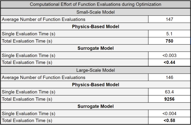
The surrogate model-based optimization framework leverages the speed and structure of surrogate models to provide quick and robust solutions to engineering optimization problems. The table from one example highlights the significant differences in computation effort required for optimization while using surrogate and physics-based models. Complex optimization algorithms require many function evaluations, and using physics-based simulators to service these evaluation requests results in a considerable computation effort. Surrogate models remove this bottleneck by providing optimization algorithms with quick and accurate function evaluations.
General Optimization
In the most general sense, mathematical optimization is the search for the “best x” given an objective function and, in most engineering applications, a set of constraints. Formally, the optimization problem is described as follows:
\(\max_x{f(x)}\ \text{subject to} \ g(x)\leq0,\)
where the goal is to find the value of \(x\) that results in the largest value of the objective, \(f()\), while still adhering to the constraint(s), \(g()\). If we now cast the problem in the context of physics-based simulation, we can think of the function and constraints as functions of the outputs of the simulator and x as the inputs to the simulator. In this context:
\(\max_x{f(\text{simulator}(x))}\ \text{subject to} \ g(\text{simulator}(x))\leq0,\)
where, in a slight abuse of notation, \(\text{simulator}()\) represents the physics-based simulation (i.e., takes in an input \(x\) and returns some simulated outputs). While this notation deviates slightly from traditional mathematical conventions, it underscores the necessity of executing the simulator to evaluate the objective or constraint functions. For the water pumping networks we introduced in the Basics of Surrogate Model Creation, we describe the elements of the optimization problem as follows:
\(\text{x: pumping speeds},\)
\(\text{simulator(): flow rates and pumping powers},\)
\(\text{f(): collector flow rate},\)
\(\text{g(): limit on total pumping power},\)
Therefore, the goal is to maximize the flow rate at the collector without exceeding the total power drawn by the system’s pumps. This optimization problem is just one example of the many that can be formulated for water-pumping networks.
Mathematical optimization underpins most of engineering. The typical engineering trade-offs are often resolved via optimization. However, optimization is very computationally costly. Most optimization algorithms require many evaluations of the objective and constraint functions. In the context of physics-based simulation, this means executing the simulator repeatedly, and due to the nature of these algorithms, these executions occur in series. Moreover, this costly endeavor may only result in a “local” maximum, an \(x\) that is better than those around it but not the absolute best. However, optimizing becomes much more attractive if we replace executing the physics-based model with a much less costly surrogate model.
Surrogate Model-Based Optimization
Suppose a surrogate model is generated (with small prediction errors). In that case, the physics-based simulation optimization problem can be reformulated as follows:
\(\max_x{f(\text{surrogate}(x))}\ \text{subject to} \ g(\text{surrogate}(x))\leq0,\)
The optimization problem is solved quicker since \(\text{surrogate}()\) is evaluated much faster than \(\text{simulation}()\). Furthermore, if the prediction errors are small (or insignificant), the solution should closely match one obtained with a physics-based simulator.
[1] and [2] describe alternative formulations of surrogate model-based optimization. All three formulations use surrogate models’ increased speed to obtain optimized answers much quicker.
Surrogate Construction and Optimization
Note that the inputs and outputs of the surrogate models will inform the set of possible optimization problems. The functions \(f()\) and \(g()\) can only be functions of the surrogate’s inputs or outputs, and optimized inputs, \(x\), must be a subset of the inputs to the surrogate. In the water-pumping networks example, we cannot, for example, have a constraint on a fluid’s temperature since the surrogate model does not predict fluid temperature. Ideally, the optimization problem formulation should occur before constructing the surrogate.
Decision and Fixed Variables
Not all of the inputs to the surrogates need to be optimized. Some may remain fixed during the optimization process. We labeled these inputs as “fixed variables.” For example, suppose we create a surrogate model of a building heating system. Undoubtedly, the ambient temperature will be a surrogate input since it is an essential variable in determining the system’s behavior. However, we should not optimize ambient temperature since we have no direct control of this variable. Nevertheless, the ambient temperature will affect any optimization done on this system. Therefore, we introduce a final iteration of the optimization problem formulation:
\(\ \text{given p} \ \max_{x_{\text{decision}}}{f(\text{surrogate}(x_{\text{decision}},x_{\text{fixed}}))}\ \text{subject to} \ g(\text{surrogate}(x_{\text{decision}},x_{\text{fixed}}))\leq0 \ \text{and} \ x_{\text{fixed}} = p, \)
where \(p\) are the values of the fixed variables. The union of \( x_{\text{decision}} \) and \( x_{\text{fixed}} \) must equal the complete input set of the surrogate model. An optimization problem set up with fixed variables is given [3].
Examples
Two examples of optimization problems are described and solved. We leveraged the framework’s speed to execute the underlying optimization algorithm several times. Each execution is seeded with a random initial guess to provide a robust final answer (we output the best result). In practice, executions can be conducted in parallel to achieve quicker results.
Example 1: Maximize Collector Flowrate with Limited Power
In this example, we maximize the collector’s flow rate and limit the pumps’ total power draw. We also optimize the pump speeds, while the pressures at the sources and collector are assumed to be fixed variables.
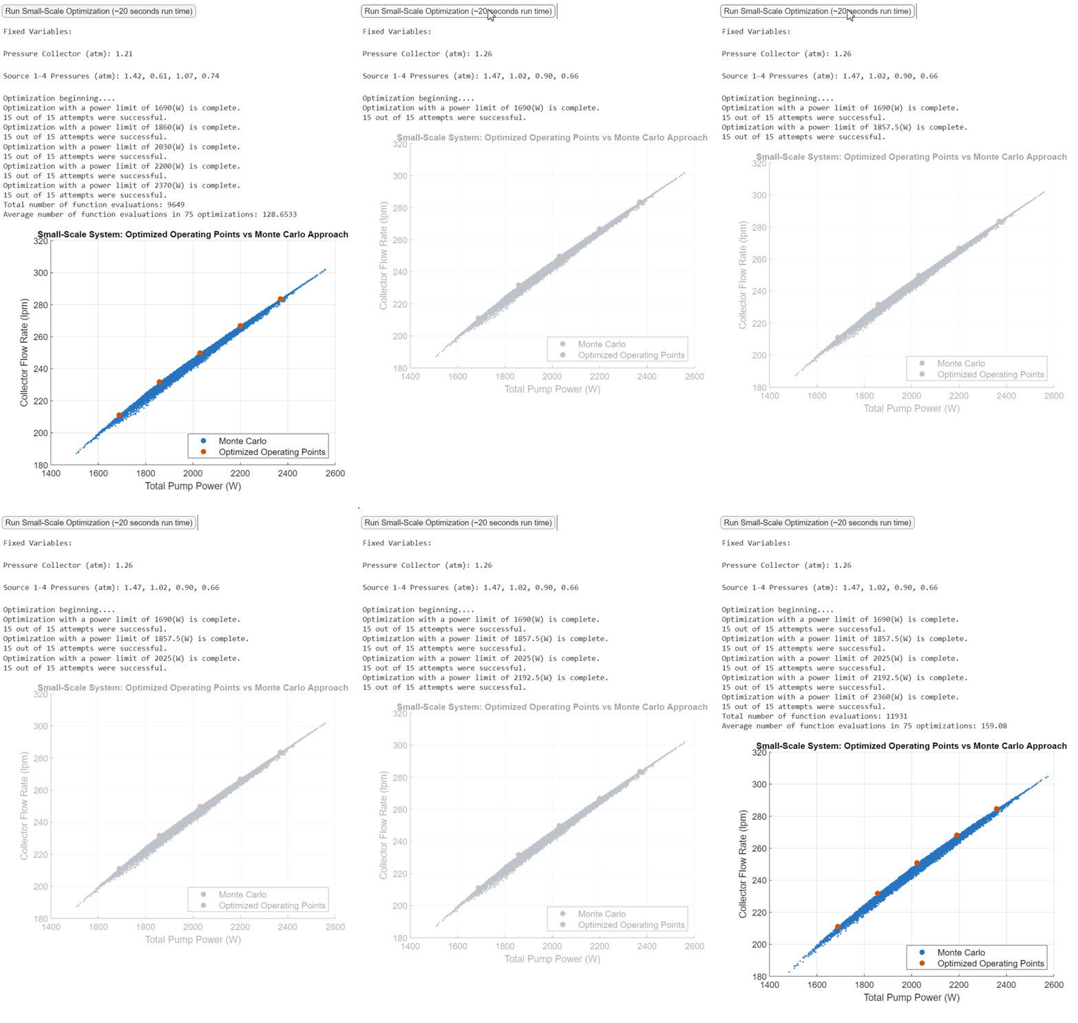
In the MATLAB executable notebook, a button is clicked to run a randomly selected scenario for the small-scale optimization. An outputted plot compares the optimized operating points at different power limits with a point cloud generated via the Monte Carlo method [4]. The optimized operating points provide the best achievable flowrate at different power limits. Note that 75 optimizations occur in the span of about 20 seconds.
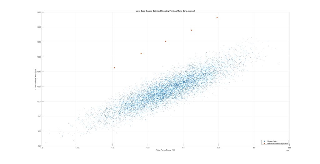
We execute the same exercise with the large-scale system. Fixed variables are not displayed but are randomly sampled with each click on the button. Again, the optimized operating points provide the best achievable flow rate at different power limits. Due to the problem’s dimension, the Monte Carlo approach is noticeably worse.
The MLP surrogate models give the optimization algorithm access to quick function evaluations. The table below highlights how surrogate models eliminate major bottlenecks in optimization algorithms. Furthermore, physics-based models become largely impractical as the optimization problem grows in complexity and dimension. In contrast, surrogate model-based optimization remains feasible and responsive.

Example 2: Maximize Profit with Limited Capacity
We now consider the case in which an organization obtains a profit for transporting water from a source to the collector. The problem is made interesting by assuming each line incurs a different profit per liter of water transported, and there is a limit on the amount of water the collector can receive. The pump speeds and collector pressures are optimized, while the pressures at the sources are assumed to be fixed variables.
In the MATLAB executable notebook, a button is clicked to run a randomly selected scenario for the small-scale optimization. An outputted plot compares the optimized profit at different flow limits with a point cloud generated via the Monte Carlo method [4]. The optimized operating points provide the best achievable profits at different collector flow rates.
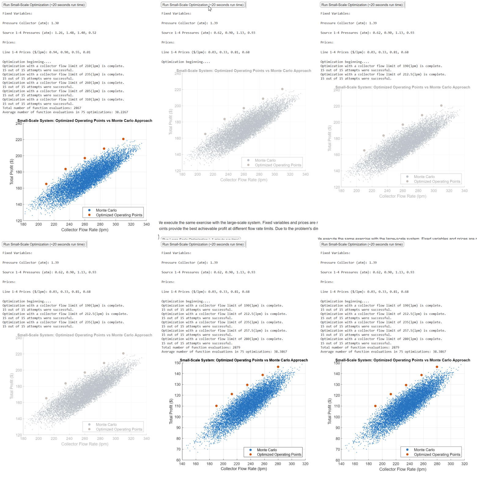
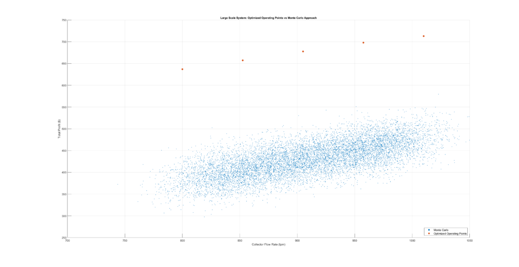
We execute the same exercise with the large-scale system. Fixed variables and prices are not displayed but are randomly sampled with each click on the button. Again, the optimized operating points provide the best achievable profit at different flow rate limits. Due to the problem’s dimension, the Monte Carlo approach is noticeably worse.
Summary
We can leverage surrogate models to perform fast and robust optimization. The MLP surrogate models give the optimization algorithm access to quick function evaluations. The article presented two examples of an optimization problem solved using small and large-scale water-pumping network systems. Finally, optimization underpins most engineering problems, and many more applications (i.e., parameter estimation, controller tuning, sensitivity analysis) share the same or very similar formulations.