Sampling with Constraints
Sampling with Constraints
Goals
- Introduce a Constrained Optimization Method: Present a practical approach for generating samples that meet specified input constraints and bounds.
- Demonstrate Practical Benefits: Use examples to illustrate how this method produces more uniformly distributed samples than traditional sampling techniques.
The article references MATLAB code and data found here.
High-Level Highlights
We introduce a straightforward method for managing input constraints, ensuring that generated samples meet all specified limits. As illustrated in the examples below, our approach produces input samples that are more uniformly distributed than those from simple sampling methods.
Input Constraints
Inputs to a system model often need to meet specific constraints to represent a valid configuration. Typically, each input has a lower and upper bound. However, some scenarios require additional constraints for physical validity. For example, specific inputs may need to satisfy a summation constraint in chemical processing system models.
In these situations, sampling methods can be adjusted ad hoc. Simple normalization or corrections can be applied to ensure that samples align with model-specific requirements. However, these ad hoc adjustments can result in skewed or sparse data sets, which may lead to inaccurate surrogate model predictions.
Proposed Constrained Optimization Approach
We present a general method for managing input constraints. This method uses constrained optimization to generate random input samples that satisfy all specified constraints and bounds. Moreover, as demonstrated in the example, our approach results in input samples that are more uniformly distributed compared to simple ad hoc methods. The accompanying MATLAB code shows how easily this approach can be adapted for different applications.
Example 1: Summation Constraint
In this example, we consider a model of a chemical processing system where we aim to sample the chemical composition of an input stream randomly. The molar fractions of each compound define the composition, and for the samples to be valid, the sum of these fractions must equal one. Therefore, we must account for this summation constraint when sampling. Additionally, we set bounds on the fraction of each compound to reflect a range of operating conditions of the chemical processing system. Ideally, the generated samples should sum to one and stay within these specified bounds.
A simple way to generate samples is to normalize random numbers within the defined bounds. The following equation demonstrates how this approach can be applied to a simple three-compound chemical stream:
\( S_1 = \mathcal{U}_{[B_{1, lower}, B_{1, upper}]}, \quad
S_2 = \mathcal{U}_{[B_{2, lower}, B_{2, upper}]}, \quad
S_3 = \mathcal{U}_{[B_{3, lower}, B_{3, upper}]} \)
S_2 = \mathcal{U}_{[B_{2, lower}, B_{2, upper}]}, \quad
S_3 = \mathcal{U}_{[B_{3, lower}, B_{3, upper}]} \)
\(\bar{S}_1 = \frac{S_1}{S_1 + S_2 + S_3}, \quad \bar{S}_2 = \frac{S_2}{S_1 + S_2 + S_3}, \quad \bar{S}_3 = \frac{S_3}{S_1 + S_2 + S_3}\)
This simple method generates samples using a uniform distribution (the code provided employs the Latin Hypercube method) based on the specified compound bounds. After generating the samples, normalization ensures their sum equals one. However, this method may produce samples that fall outside the prescribed bounds. The proposed constrained optimization approach only generates valid samples within the specific bounds.
We generate samples for a chemical stream with the molar fraction ranges listed in the table below to highlight the differences between the two methods.

The figure below compares samples generated using the simple normalization approach with those produced by the constrained optimization approach. We generated 5,000 samples with both methods and analyzed their distributions. Black dashed lines indicate the nominal limits (as shown in the table), while blue dashed lines represent the ideal uniform probability.
It’s important to note that the simple method generates samples outside the specified bounds for compounds 1 and 2. Additionally, compound 3 shows a lack of coverage at the edges of its possible range using the simple normalization approach. The resulting distributions also appear more Gaussian than uniform. In contrast, the constrained optimization method only produces samples within the defined bounds, and its distribution more closely resembles the ideal uniform distribution.
We have provided the Matlab code used to compare these two approaches here.

Example 2: Uniformity in Composite Parameters
In this example, we explore a case where a system model has a critical composite parameter that must be considered when randomly sampling the system. We define a composite parameter as a parameter that is not an input to the system model but is nevertheless important in determining the overall system behavior. We assume that the value of this parameter can be computed analytically from the system model’s inputs.
For instance, consider a water treatment plant operating in a steady state with multiple input streams. While the inputs to the model may include the flow rates of each input stream, the output flow rate (the amount of water being treated) is not included as an input. However, the output flow rate is crucial, significantly affecting the system’s behavior and performance. Therefore, when generating samples for surrogate model applications, it is beneficial that the resulting output flow rates are distributed uniformly across the entire possible range.
The most straightforward sampling strategy does not take the composite parameter into account. In the case of the water treatment plant, the outlet flow rate (denoted as \(O\)) is computed by the sum of the inlet flow rates (denoted as \(I_i\)) as follows:
\(I_1 = \mathcal{U}_{[B_{1, lower}, B_{1, upper}]}, \)
\(I_2 = \mathcal{U}_{[B_{2, lower}, B_{2, upper}]}, \)
\(I_3 = \mathcal{U}_{[B_{3, lower}, B_{3, upper}]} \)
\(O = I_1 + I_2 + I_3\)
As demonstrated below, this basic strategy can lead to an undesirable distribution of the composite parameter. Conversely, the proposed constrained approach can be tailored to produce more favorable distributions.
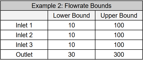
To highlight the differences between the two methods, we generated samples for the water treatment plant using flow rate ranges listed in the table below. We configured the constrained approach to prioritize the outlet flow rate distribution over the inlet flow rate distributions.

The figure below compares samples generated using the simple sampling approach with those produced by the constrained optimization approach. We generated 5,000 samples using both methods and analyzed their distributions. Black dashed lines indicate the nominal limits (as shown in the table), while blue dashed lines represent the ideal uniform probability.
The simple sampling method produces an outlet flow rate distribution that resembles a normal distribution, with fewer samples at the extremes of the possible outlet flow rates. This poor data quality can lead to poor prediction performance of the surrogate model when flow rates are close to these bounds.
In contrast, the proposed approach creates an ideal uniform distribution of the outlet flow rate. As a result, when the model is sampled with the generated inputs, there will be no sparsity around any outlet flow rate. This improves the surrogate model’s ability to capture the complete behavior of the system.
We have provided the Matlab code used to compare these two approaches here.

Example 3: Constrained Composite Parameters
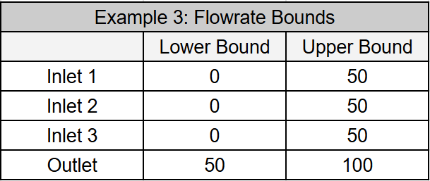
In this final example, we revisit Example 2. We now treat the input parameters (inlet flow rates) and the composite parameter (outlet flow rate) as equally important without prioritizing one over the other. The table below presents new parameter bounds. Note that some combinations of inlet flow rates may produce outlet flow rates that fall outside these defined bounds.

A straightforward strategy for managing the outlet flow rate bounds is to sample the inlet flow rates as usual. If the resulting outlet flow rate falls outside the defined limits, we add an adjustment to each inlet value to make the adjusted resulting outlet flow rate within bounds. For more details, please refer to the provided code.
As before, we generated 5,000 samples to compare the different approaches. In this case, the constrained method was configured to treat all parameters equally. The black dashed lines indicate the nominal limits (as shown in the table), while the blue dashed lines represent the ideal uniform probability.
The simple sampling method resulted in skewed samples, with relatively few inlet flow rate samples near the edges of their bounds. The outlet flow rate distribution also had low sample counts in the middle of its range. In contrast, the proposed constrained approach produced samples where all distributions closely resembled the ideal uniform distribution.
We have included the Matlab code used to compare these two approaches here.

Summary
We introduced a constrained optimization approach for generating input samples that meet specific constraints and compared it to simple sampling methods. The constrained optimization method produced input samples that satisfied the defined constraints and resulted in a more uniform distribution. In general, skewed and sparse datasets can result in poor surrogate model prediction performance. The provided MATLAB code demonstrates this approach can be easily configured for various applications.