DWSIM Surrogate Creation
DWSIM Surrogate Creation
Goals
- Goal #1: Introduce key concepts of surrogate models in the context of DWSIM, an open-source chemical process simulator
- Goal #2: Demonstrate three surrogate model creation examples
The article references MATLAB code and DWSIM models notebook found here.
High-Level Highlights
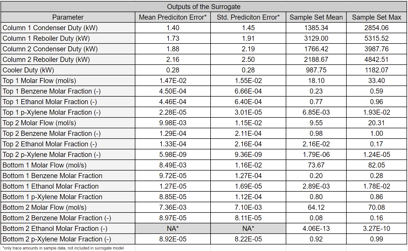
We construct surrogate models of chemical processing models created in DWSIM. As shown previously in Basics of Surrogate Model Creation, surrogate models obtain results nearly identical to physics-based models but in a fraction of the time. The tables below display the accuracy and performance of a surrogate of an extractive distillation chemical process model.

DWSIM
DWSIM is an open-source chemical process simulator. The simulator has a large and expanding set of unit operations, thermodynamics models, utilities, and tools. The DWSIM homepage provides much more information and a free software download.
Surrogate Creation
As shown previously in Basics of Surrogate Model Creation, surrogate models obtain results nearly identical to physics-based models but in a fraction of the time. The speed and accuracy of surrogate models accelerate engineering workflows such as optimization, parameter estimation, and anomaly detection. One can effectively remove the physics-based model bottleneck in optimization and analysis use cases by initially investing time and computational resources in sampling and surrogate model generation. Basics of Surrogate Model Creation walks the reader through the surrogate creation process. We will focus primarily on presenting results here but refer to other pages for additional details.
Example 1: A Simple Distillation Column
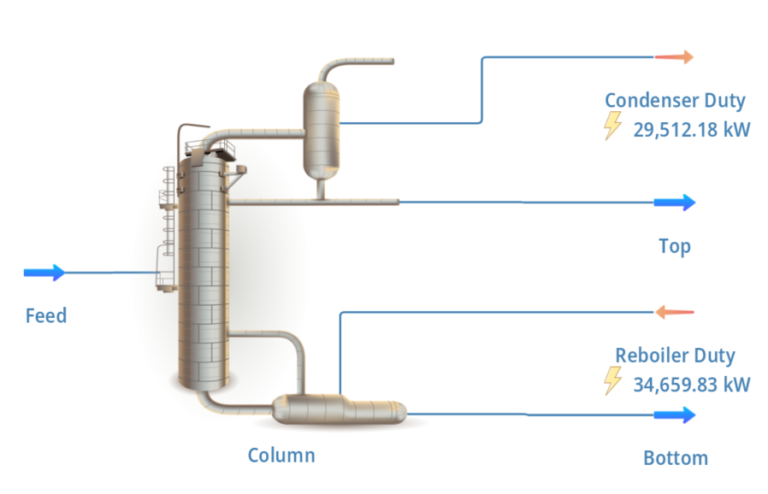
Distillation is a process of separating two or more components from a chemical mixture. It is a vital operation in chemical processing. Our first example demonstrates a surrogate model for a simple distillation column. Examples 2 and 3 expand upon this example and present processes with multiple and more complex distillation processes.
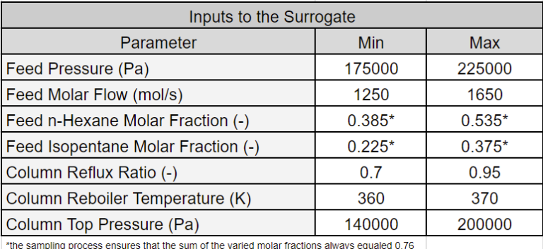
The table below lists the surrogate model inputs and their bounds. Note that only the molar fractions of two feed components were varied (five components in total), and the sum of these molar fractions was the same in all samples collected to ensure that molar fractions remained constant for the unvaried components. The sampling algorithm can be easily modified to include variations of all feed components.
The DWSIM model was executed with input parameters randomly generated from the bounds shown in the table above (see the sampling script for further details). We trained a surrogate model with a training set of 1250 samples and a validation set of 125 samples. The performance of the surrogate model was evaluated with a test set of 2500 samples (for demonstration purposes, the test set was much larger than typical). Performance metrics were generated using the test set. Data samples found in a test set are reserved and not used during model training. Therefore, prediction errors generated using a test sample set give an unbiased assessment of the performance of the surrogate model. Refer to [2] for definitions of the different sets.
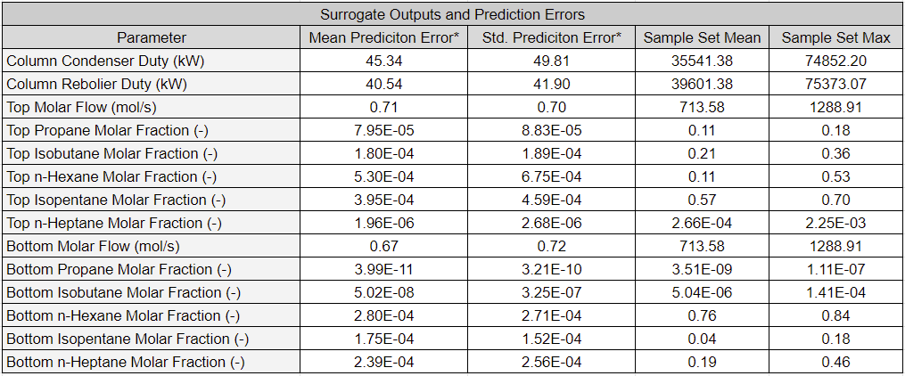
The table below presents the surrogate model outputs and their prediction errors. Recall from Basics of Surrogate Model Creation that prediction errors are the difference between the output parameter values computed by the physics-based and surrogate models. Therefore, prediction errors measure the surrogate model’s ability to emulate the physics-based model. In addition to prediction errors, the mean and max of the generated samples are also displayed.
Note that most errors are several orders of magnitude smaller than the mean of the sampled parameters. Therefore, prediction errors are negligible for most practical applications as the prediction errors are much smaller than the parameter’s value.
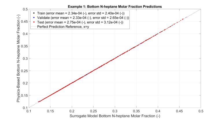
The figure below gives the reader a visual assessment of the surrogate model’s accuracy. It plots the surrogate predictions for Bottom n-Heptane Molar Fraction against those computed with the DWSIM model for the training, validation, and testing sets. MLPs tend to be overfitted, resulting in smaller errors for the training set. Therefore, as discussed above, the metrics from the testing set provide a more accurate indication of errors when predicting configurations not present in the sampled set. A complete set of figures is provided here.
Surrogate model evaluations (inference) occur much quicker than executing a physics-based model. The table below presents a computational time comparison between DWSIM model executions and surrogate model evaluations. As shown in Surrogate Model-Based Optimization and Parameter Estimation via Profile Likelihoods, the increase in speed can be leveraged to enable and accelerate vital workflows.

Example 2: Extractive Distillation
This example presents a surrogate model for an extractive distillation system, which is more complex than the one in Example 1. In extractive distillation, an entrainer is introduced to an azeotropic mixture (the mixture components have similar boiling points) to change the component’s relative volatility. The components and entrainer are then separated via distillations. The entrainer is typically recycled back into the process after it is separated from the feed. The image below displays the flow sheet of the extractive distillation system used in this example.
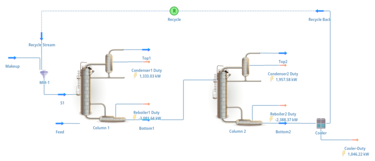
The DWSIM model (with some modifications) was constructed by following the instructions presented in this video [3]. The DWSIM model, the surrogate model, and sampled data sets can be found here.
The table below lists the surrogate model inputs and their bounds. The feed stream consists of two components. During the sampling process, the molar fractions of the components were varied, but their sum always equaled unity.
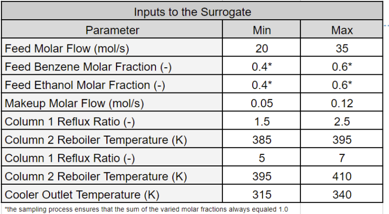
The DWSIM model was executed with input parameters randomly generated from the bounds shown in the table above. We trained a surrogate model with a training set of 2000 samples and a validation set of 150 samples. A test set of 2500 samples was used to assess performance (for demonstration purposes, the test set was much larger than typical). Refer to [2] for definitions of the different sets.
The table below presents the surrogate model outputs and their prediction errors. As in Example 1, most errors are several orders of magnitude smaller than the mean of the sampled parameters.

Similar to Example 1, a complete set of truth plots for this example is provided here.
The table below compares the computational time between DWSIM model executions and surrogate model evaluations.

Example 3: Natural Gas Processing Unit
The final example constructs a surrogate of a natural gas processing unit. This unit consists of three distillation columns and auxiliary mechanical equipment. Four material streams are created from a single incoming feed stream. The surrogate model predicts the make-up of the four outputted material streams and the energy expenditure of the distillation columns and auxiliary equipment. The image below displays the flow sheet of the natural gas processing unit used in this example.
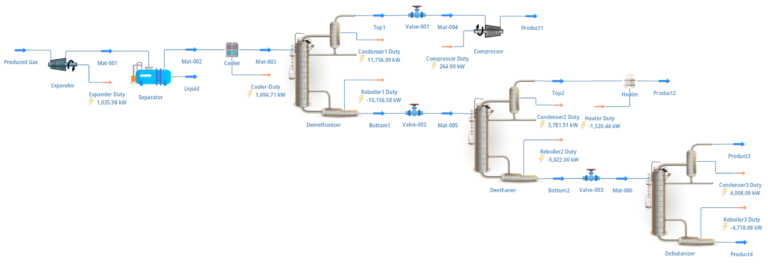
The DWSIM model used in this example was a modification of an example model included in the DWSIM software download (“Natural Gas Processing Unit.dwxmz”). The DWSIM model, the surrogate model, and sampled data sets can be found here.
The table below lists the surrogate model inputs and their bounds. Note that only the molar fractions of three feed components were varied (9 components in total), and the sum of these molar fractions was the same in all samples collected to ensure that molar fractions remained constant for the unvaried components. The sampling algorithm can be easily modified to include variations of all feed components.
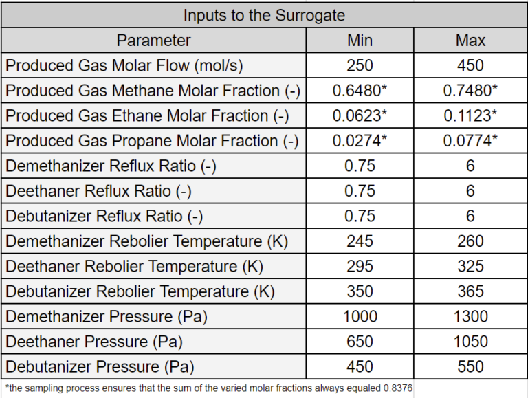
The DWSIM model was executed with input parameters randomly generated from the bounds shown in the table above. We trained a surrogate model with a training set of 2500 samples and a validation set of 250 samples. A test set of 2500 samples was used to assess performance (for demonstration purposes, the test set was much larger than typical). Refer to [2] for definitions of the different sets.
The table below presents the surrogate model outputs and their prediction errors. As in Example 1, most errors are several orders of magnitude smaller than the mean of the sampled parameters.
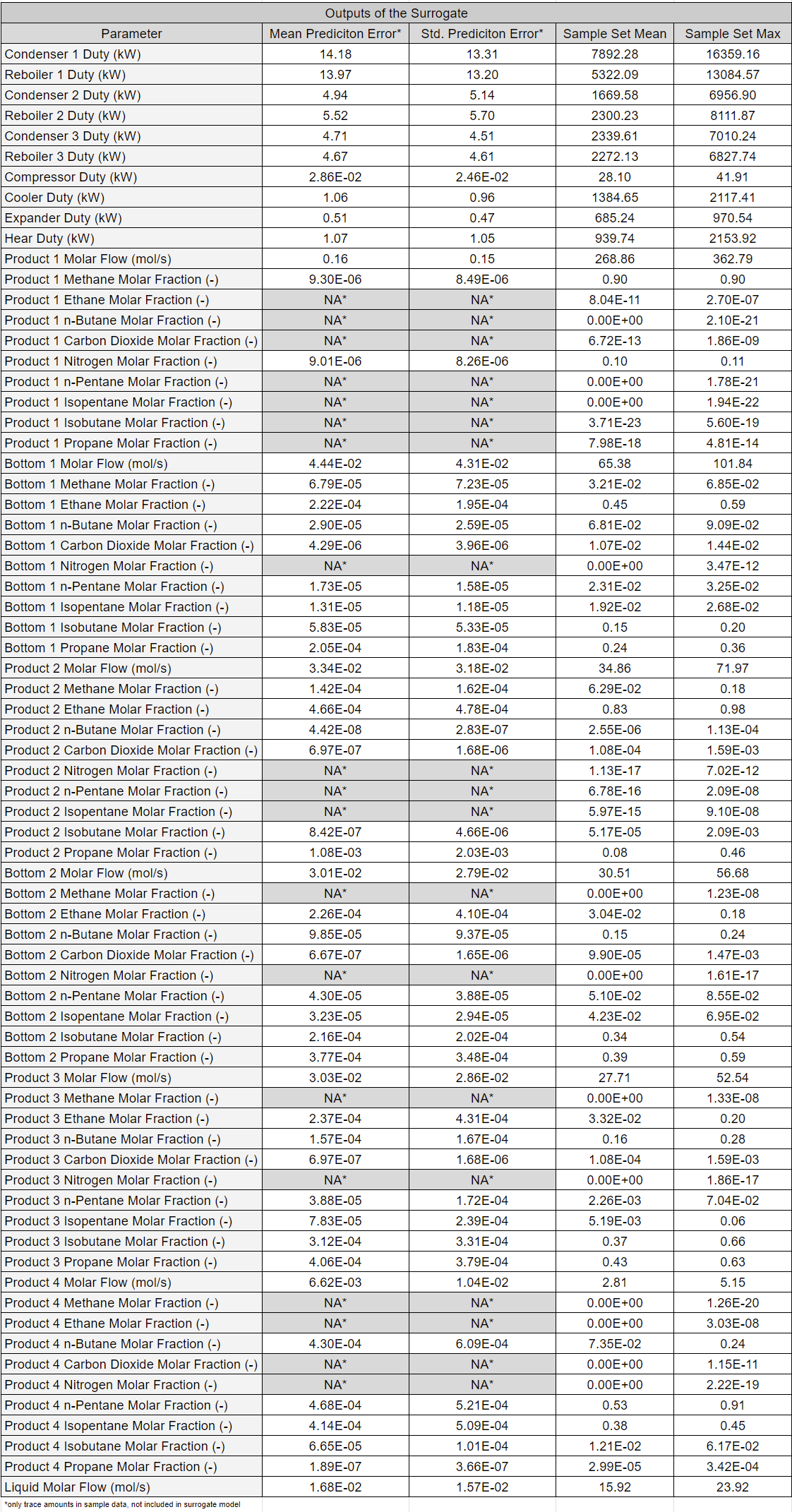
Similar to Example 1, a complete set of truth plots for this example is provided here.
The table below presents a computational time comparison between DWSIM model executions and surrogate model evaluations.

Summary
We construct surrogates of chemical processing models created in DWSIM. As shown previously in Basics of Surrogate Model Creation, surrogate models obtain results nearly identical to physics-based models but in a fraction of the time. In future work, we will leverage the speed and flexibility of these surrogate models to demonstrate fast system-level optimization and parameter estimation.