Anomaly Detection

Goals

  • Anomaly Detection: Describe what anomaly detection is and its importance.
  • Sampling and Data Comparison Methods: We present two approaches for anomaly detection, both of which leverage the speed and flexibility of surrogate models.
  • Walk-Through: Offer a simple, step-by-step guide of an example using both approaches.

The article references a MATLAB executable notebook, code, and Simulink models found here.

High-Level Highlights

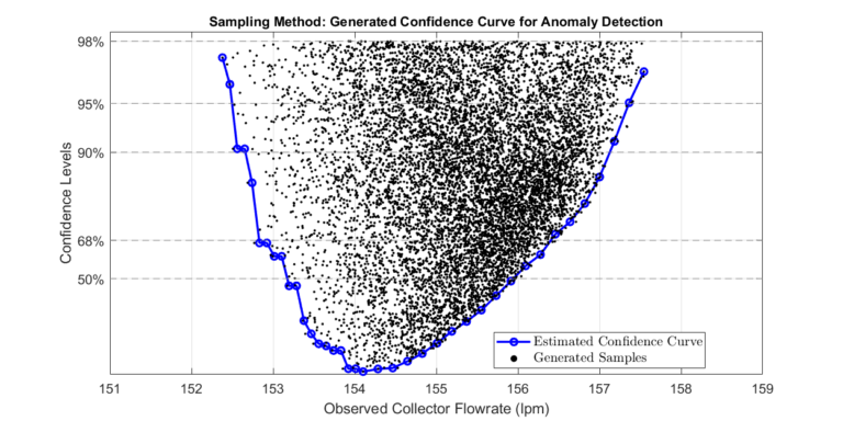
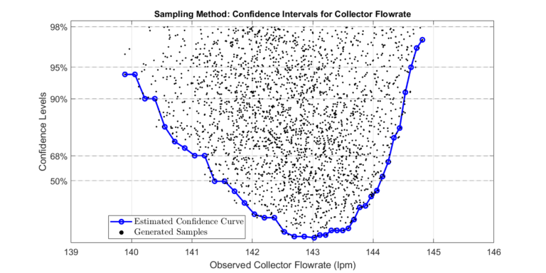
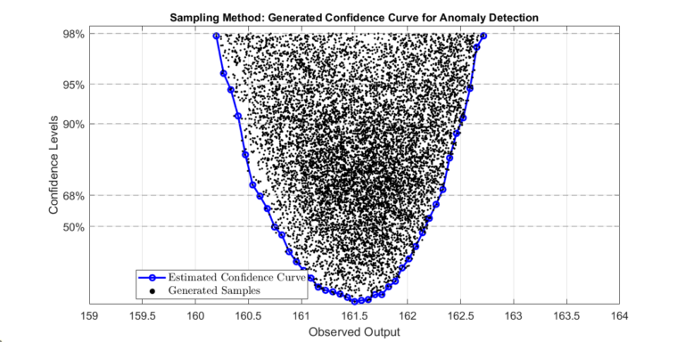
Quickly detecting anomalous events is essential for safety-critical or highly optimized systems. Anomalous events may give the first indication of a system fault, failure, or mode change. We present two methods for computing confidence levels of a model’s output. When used effectively, confidence levels can help you determine when an anomalous event occurs, thereby enhancing the safety and efficiency of systems. The plot below shows the result of the sampling method, a confidence curve of a system’s output. Both methods leverage the flexibility and speed of surrogate models to produce confidence curves quickly and robustly.
Anomaly Detection

As noted in Optimization Under Uncertainty, some inputs to a simulation model may not be fully known or controlled. The values of these parameters are typically estimated or tuned to ensure the simulation model is accurate. However, any uncertainty in model parameters will cause uncertainty in the model’s output. In Optimization Under Uncertainty, we used confidence bounds to establish system performance predictions under uncertainty. Given some confidence level, we can establish the range of expected system output.
Anomaly detection is a natural extension of this analysis. It determines when the system’s behavior falls outside the expectation, that is, when the simulation model fails to predict the observed behavior. Detecting anomalous events is vital for autonomous systems or any tightly controlled system since accurate predictions are necessary for model-based actions and decisions. Furthermore, an anomalous event can be caused by a system failure, fault, or mode change. Therefore, anomaly detection may be the first step in uncovering a more significant issue with the system.
Understanding the concept of confidence levels is key to implementing anomaly detection. In the previous section, we presented a plot that displays the computed confidence levels of a system’s output. These levels help us establish the expected value of the system’s output. Any values that fall outside of this range would be considered anomalous, indicating a deviation from the system’s expected behavior.

Known and Uncertain Variables

In Surrogate Model-Based Optimization, we established the difference between decision and fixed variables. Here, we introduced a similar classification of model inputs: known and uncertain variables. Known variables are inputs to the model that are assumed to be perfectly known—for example, control parameters such as motor speeds or actuator voltages. Uncertain variables are inputs to the model that need to be estimated or are not completely known. Therefore, we cannot establish the exact values of these variables. However, as seen in Optimization Under Uncertainty, we can compute ranges of their possible values. As discussed in Surrogate Model-Based Optimization, the union of \( x_{\text{known}} \) and \( x_{\text{uncertain}} \) must equal the complete input set of the model. Therefore, an input to the model is either known or uncertain. In the context of surrogate models:
\( \text{surrogate}(x) = \text{surrogate}(x_{\text{known}},x_{\text{uncertain}}) \)
Note that the surrogate model’s output will be uncertain since the uncertain variables, \( x_{\text{uncertain}} \), can take a range of values. The following sections will present two approaches to computing confidence levels for the surrogate’s output.

Sampling Approach

The sampling approach utilizes the parameter estimation confidence levels from Parameter Estimation via Profile Likelihoods. We start by estimating the parameter via profile likelihood, enabling us to compute the confidence levels of various parameter configurations. Similar to Optimization Under Uncertainty, we consider the set of all possible uncertain variable values for a given confidence level \( \alpha \),
\(P_\alpha = \{ x_\text{uncertain}^1,x_\text{uncertain}^2,\dots.\}. \)
We will approximate the infinite set \(P_\alpha \) with a finite set \(\bar{P}_\alpha \) ,
\( \bar{P}_\alpha = \{ x_\text{uncertain}^1,x_\text{uncertain}^2,\dots x_\text{uncertain}^n\}. \)
The finite set \( \bar{P}_\alpha \) is constructed by iteratively computing the likelihoods of randomly generated sets of fixed variables. Any \( x_\text{uncertain}^i \) that achieves a minimal likelihood (based on the selected confidence level \( \alpha \) and the number of uncertain variables [1]) is placed into the set \( \bar{P}_\alpha \). The process is repeated in a loop until \( \bar{P}_\alpha \) is of the desired size. The likelihoods of \( x_\text{uncertain}^i \) are also recorded in \( \bar{S}_\alpha \).
Next, a set of inputs to the surrogate model can be created by augmenting the members of \( \bar{P}_\alpha \) with a known input, \( x_{\text{known}} \):
\( X = \{ (x_\text{known}, x_\text{uncertain}^1),(x_\text{known}, x_\text{uncertain}^2),\dots (x_\text{known}, x_\text{uncertain}^n)\} \).
All members of \( \bar{P}_\alpha \) are augmented with the same \( x_{\text{known}} \) since confidence bounds are computed at a specific operating point. The surrogate model is evaluated over all \( X \):
\( \text{surrogate}(X) = Y = \{y_1,y_2,\dots,y_n\} \).
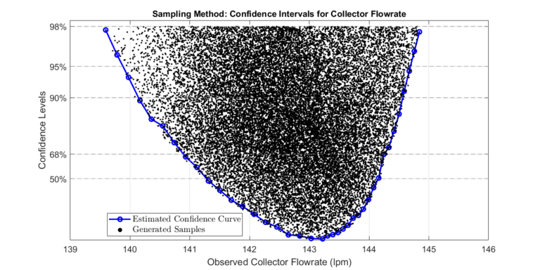
The sets \( Y\) and \( \bar{S}_\alpha \), likelihoods computed during the creation of \( \bar{P}_\alpha \), are used to calculate confidence levels of the surrogate model output. The plot below visualizes the approach. Note that the accuracy of the estimate confidence curve will increase with more samples. If the system’s operating point changes, we repeat the process to compute confidence levels at the new operating point.
This approach is feasible due to the efficiency and flexibility of surrogate models. The Results section demonstrates that the surrogate model can evaluate a batch of tens of thousands of points in less than a second.

Data Comparison Approach

This approach uses stored/historical data to determine the confidence levels of future outputs. Values of the unknown modeling parameters are estimated from the stored data by maximizing the likelihood function. We then redo the same estimation process while enforcing an additional constraint that the output of the surrogate model equals a selected value. Like constructing profile likelihood curves, the difference between the two likelihood values determines the confidence level of observing the selected value. Recall from Parameter Estimation via Profile Likelihoods that profile likelihood curves of unknown parameters were constructed by maximizing the likelihood function for each parameter of interest while holding a single parameter fixed at specific values. For this approach, we hold a single output fixed at specific values while maximizing the likelihood function.
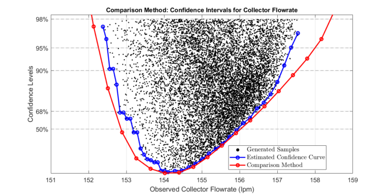
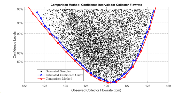
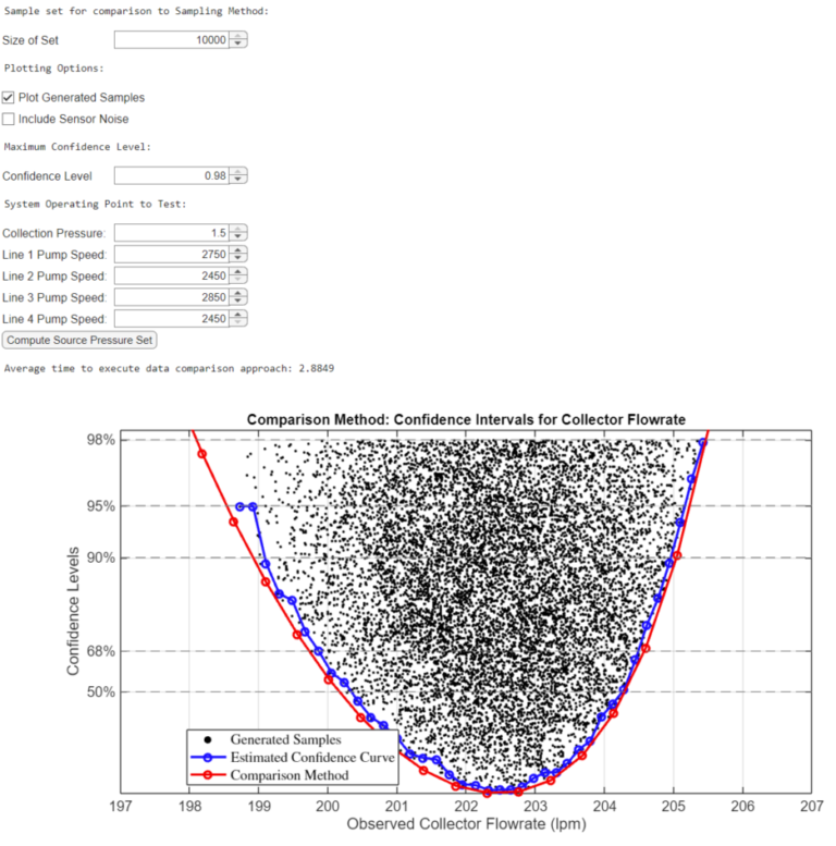
The plot below compares the sampling approach to the data comparison approach. It’s important to note that the data sampling approach approximates the data comparison approach. However, the data comparison approach stands out for its scalability, as it doesn’t rely on generating samples over a parameter space. In contrast, the sampling approach can quickly become unmanageable as the number of parameters increases. As demonstrated in Surrogate Model-Based Optimization, the data comparison approach is efficient for larger systems since it utilizes an optimization algorithm for parameter estimations. Furthermore, as shown in Surrogate Model-Based Optimization, optimization methods outperform Monte Carlo-based methods as the dimension of the system increases.

Sensor Noise

Both methods can be modified to include sensor noise in the computed confidence levels. In the sampling approach, set \( Y \) is modified to add sensor noise to the surrogate model output. Moreover, the optimization constraint in the data comparison approach can be relaxed to include sensor noise.

Example: Sampling Approach

In this section, we walk through an example to compute the confidence levels of an output of a system. We will use the small-scaled water pumping network described in Basics of Surrogate Model Creation. Our goal is to determine confidence levels for the observed collector flow rate.

Step 1: Estimate Unknown Model Parameters
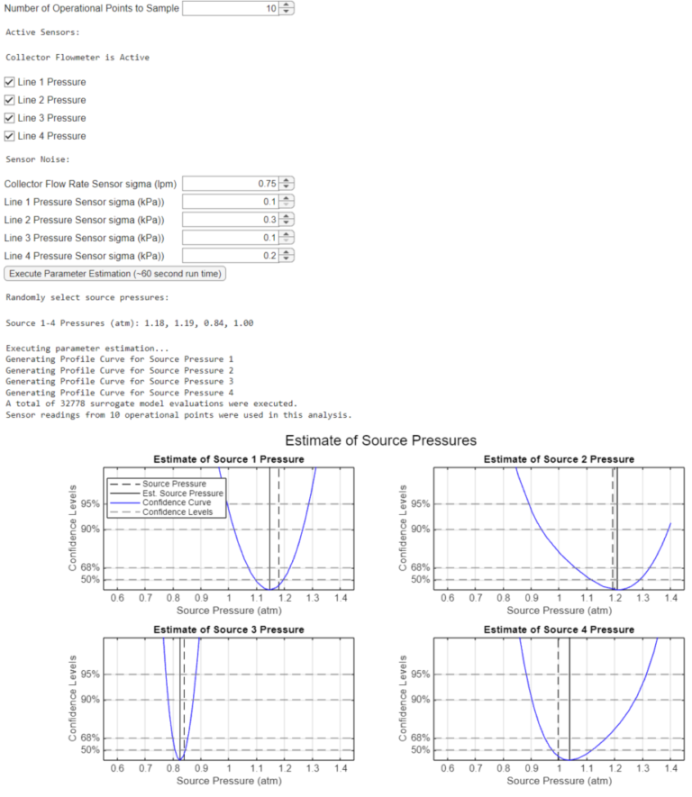
First, we perform the parameter estimation procedure detailed in Parameter Estimation via Profile Likelihoods. The procedure results in estimates and confidence levels for all four source pressures. Source pressure is uncertain for this system since it is not directly controlled or observed. The confidence levels will be used to construct a set \( \bar{P}_\alpha \) in the following step.
The MATLAB executable notebook provides a GUI Interface (described in detail in Parameter Estimation via Profile Likelihoods) where users can perform parameter estimation. The image below captures the GUI and the output from the process. For this example, we assume the collector flowmeter to be active. The user can select which pressure sensors are active.

Step 2: Compute Source Pressure Set

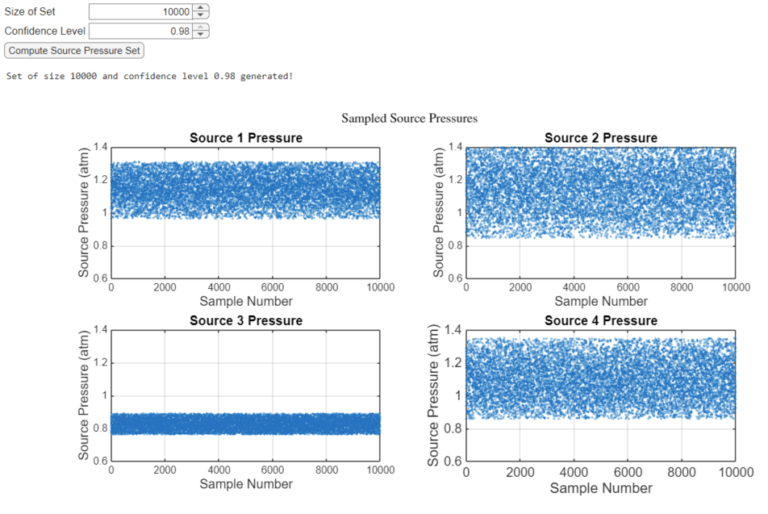
Once we compute the confidence intervals, a set \( \bar{P}_\alpha \) can be constructed. A set of the specified size is computed in which members fall within the specified confidence level. We plot the gathered set for visual inspection.

The image below captures the GUI and the output from the process. 
Step 3: Determine Confidence Intervals of Collector Flowrate
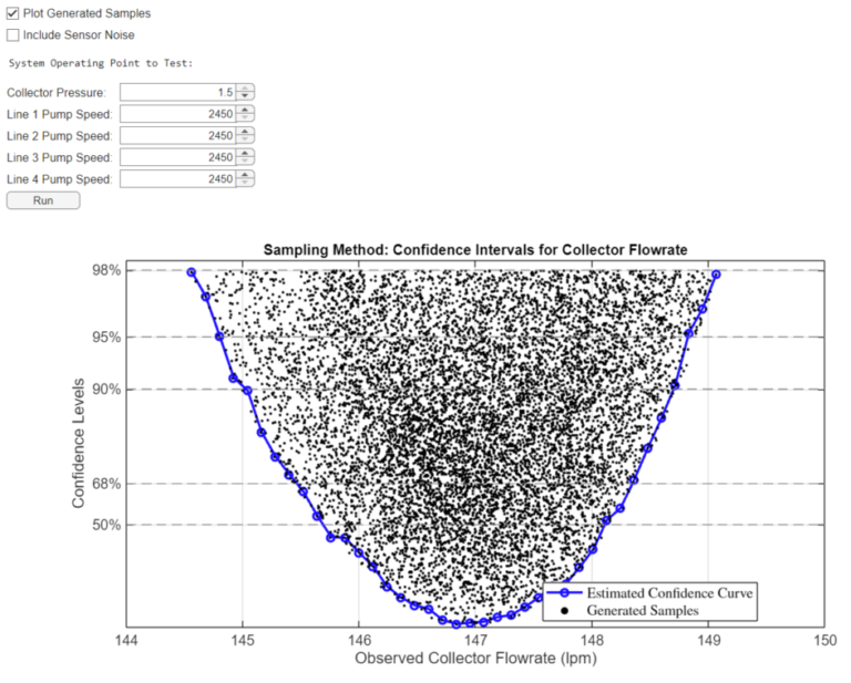
The water pumping network has five known variables: the collector pressure and the pumping speed for each line. Once the operating point is defined, we evaluate the surrogate model at each member of the generated set \( \bar{P}_\alpha \). We sort the resulting outputs by their value and the likelihood of the associated uncertain variables. Once sorted, the estimated confidence levels of the modeling output can be computed. The plot below visualizes the process’s final result.
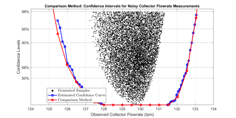
The workflow can incorporate the sensor noise of the observed output, including sensor noise results in broader confidence bounds to accommodate the larger range of possible (noisy) outputs.
The MATLAB executable notebook provides a GUI where the user can define the operating point and select between different plotting options. The image below captures the GUI and the output from the process. 

Example: Data Comparison Approach

We walk through the same example as in the previous section.

Step 1: Collect Historical Data and Estimate Unknown Parameters

First, we perform the parameter estimation procedure detailed in Parameter Estimation via Profile Likelihoods. The procedure results in estimates and confidence levels for all four source pressures. Source pressure is uncertain for this system since it is not directly controlled or observed. The confidence levels will be used to construct a set \( \bar{P}_\alpha \) in the following step.
The MATLAB executable notebook provides a GUI Interface (described in detail in Parameter Estimation via Profile Likelihoods) where users can perform parameter estimation. The image below captures the GUI and the output from the process. For this example, we assume the collector flowmeter to be active. The user can select which pressure sensors are active.

Step 2: Compute the Profile Curve of the Output

We use the historical data generated in the previous step to compute a profile curve of future collector flow rates. 

The plot compares the two approaches. Note that the comparison approach gives wider confidence bounds since the sampling method approximates confidence levels. 

The MATLAB executable notebook provides a GUI where the user can define the operating point, select between different plotting options, and set the sampling set for comparison. The image below captures the GUI and the output from the process. 
Results

Speed

As mentioned above, both methods leverage the speed of surrogate models. In Basics of Surrogate Model Creation, we demonstrated that surrogate models are much faster than their physics-based counterparts. This speed advantage is magnified when model evaluations are executed in batches. In the image below, the surrogate model performs tens of thousands of evaluations in under a second. The sampling approach presented above heavily leverages a surrogate model’s speed and flexibility.
In addition, in Surrogate Model-Based Optimization, we demonstrated that surrogate models accelerated and robustified constrained optimization. We exploited these advantages when implementing the data comparison approach. Note that the second walk-through example shows that the comparison method only takes a few seconds to complete. Therefore, a real-time assessment of anomalous events is possible in more efficient and realistic deployments.

Including Sensor Noise

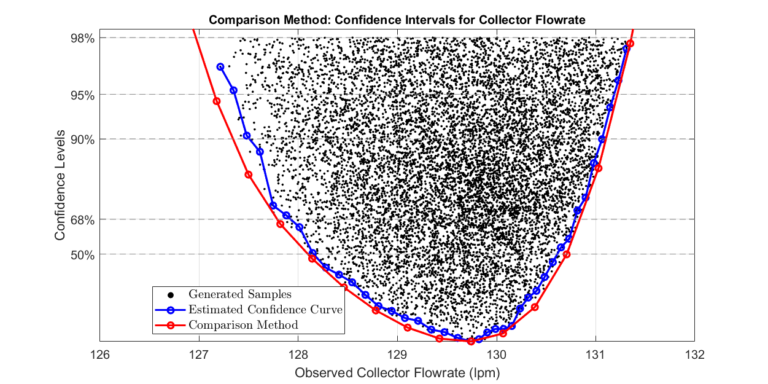
Since the observed output will be noisy, any anomaly detection algorithm should be able to incorporate sensor noise. The two plots below illustrate that both methods can do just that. The first plot displays the confidence curves when no sensor noise is considered. The second plot displays results when a sensor model of \( \mathcal{N}(0,0.75^2)\) (lpm) is assumed for the collector flowmeter.

Sparse Samples

Using sparse samples for the sampling methods reduces the accuracy of the approach. The data comparison approach is the correct path to achieving scalable results. However, the sampling approach remains implementable for small systems and is a great way to test the data comparison approach. The plot below compares the estimated confidence curve when 2,500 and 25,000 samples are available for confidence curve estimation.

Asymmetrical Results

Though most confidence levels are symmetrical, some are not. Asymmetrical results highlight the nonlinear nature of the underlying system. Instead of conducting rigorous analysis, operators may be tempted to add Gaussian noise to a physics-based model’s output to account for uncertainty. However, asymmetrical results highlight the dangers of this simple approach. Furthermore, it is challenging to translate uncertainty in modeling parameters to uncertainty in modeling outputs without rigorous analysis. Therefore, adding Gaussian noise will likely overestimate or underestimate the uncertainty in the model’s output.

Multiple Outputs

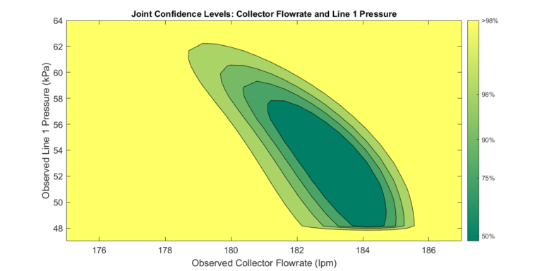
The methods presented above can be modified to include multiple outputs. The plot below displays the confidence levels for the collector flow rate and line 1 pressure. The 2-D confidence curves result in interesting relationships between the outputs and give a richer context for anomaly detection.

Summary

Identifying anomalous events is vital for safety-critical or highly optimized systems. These events are often the first sign of a system fault, failure, or mode change. We have introduced two practical methods for computing the confidence levels of a model’s output. An output’s confidence levels are used to determine the likelihood of anomalous events. Both methods leverage the flexibility and speed of surrogate models to produce confidence curves quickly and robustly.

References