Optimization Under Uncertainty
Optimization Under Uncertainty
Goals
- Connect the Bridge between Parameter Estimation and Optimization: Discuss why a robust and accurate parameter estimation is essential to execute reliable optimization.
- Optimization Under Uncertainty: Reformulate an existing optimization framework to utilize profile likelihood confidence intervals explicitly.
- Walk-Through: Offer a simple, step-by-step guide to performing optimization under uncertainty
The article references a MATLAB executable notebook, code, and Simulink models found here.
High-Level Highlights
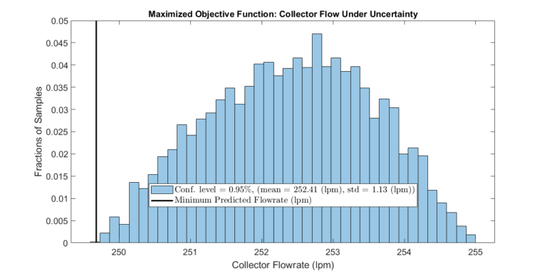
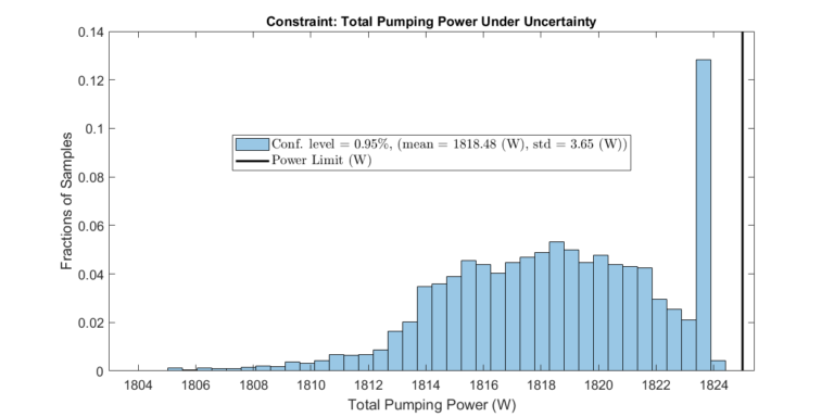
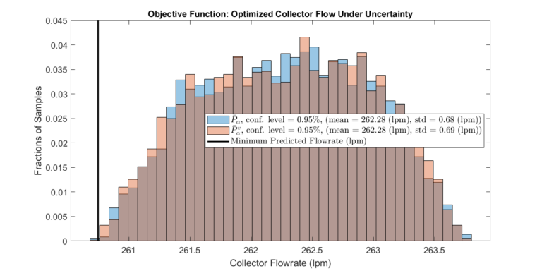
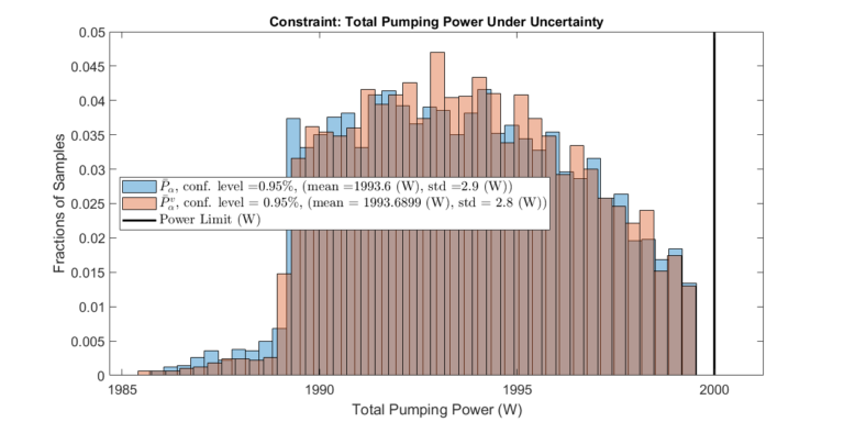
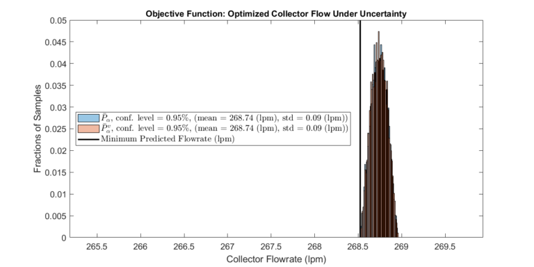
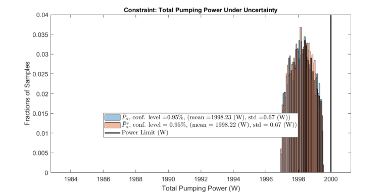
We join the parameter estimation approach introduced in Parameter Estimation via Profile Likelihoods and the surrogate model-based optimization framework discussed in Surrogate Model-Based Optimization to achieve an optimization solution under uncertain modeling parameters. Specifically, we explicitly use the parameter estimation’s confidence intervals to perform constrained optimization over a distribution of possible outcomes. The plots below summarize the result of the approach. The “worst-case scenario” is accurately predicted. At the same time, the imposed constraint is satisfied for all evaluated cases. As discussed in previous articles for other workflows, this workflow relies on many system model evaluations and only becomes feasible using surrogate models and surrogate model-based optimization techniques.
Optimization Under Uncertain Fixed Variables
The optimization framework introduced in Surrogate Model-Based Optimization distinguishes between decision and fixed variables. Fixed variables are surrogate model inputs that are not directly controlled but are essential to describe the system’s behavior. For example, ambient temperature would be a fixed variable in a building’s heating system model. However, fixed variables may need to be estimated and, in some cases, only partially known. That is, the exact value of some fixed variables may not be available. As a result, the optimized system’s performance will deviate from its predicted behavior.
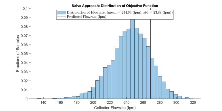
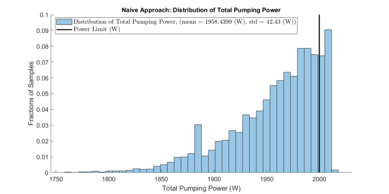
Consider the small-scaled optimization problem given by Example 1 in Surrogate Model-Based Optimization. Suppose the source pressures’ estimates (lines 1-4) are 1.0 atm but uncertain. Let’s assume the source pressures can take on a range of values with a minimum and maximum of 0.8 atm and 1.2 atm, respectively. Further, we shall constrain the total pumping power to under 2000 Watts. We then optimize only considering the nominal case where pressures equal 1.0 atm. The first plot shows how the actual collector flow rate will deviate from the predicted flow rate when pressures are allowed to take values different from the nominal case. Since we only considered the nominal case, the resulting system performance cannot be accurately assessed. Furthermore, the second plot shows that the system will violate the pumping power constraint under some off-nominal source pressures (about 15 percent of cases).
These findings underscore the inherent unpredictability and potential for undesirable outcomes stemming from uncertainty in fixed variables. In the next section, we incorporate this uncertainty into the optimization framework to produce more robust and reliable results.
Reformulate the Optimization Framework
We now reformulate the surrogate model-based optimization framework introduced in Surrogate Model-Based Optimization to explicitly consider uncertainty in fixed variables. Recall we formulated the surrogate model-based optimization problem as follows:
\(\ \text{given }p, \ \max_{x_{\text{decision}}}{f(\text{surrogate}(x_{\text{decision}},x_{\text{fixed}}))}\ \text{subject to} \ g(\text{surrogate}(x_{\text{decision}},x_{\text{fixed}}))\leq0 \ \text{and} \ x_{\text{fixed}} = p.\)
where \(f()\) is the objective function to maximize, \(g()\)describes a set of constraints, \(x_{decision}\) are the inputs to be optimized, and \(x_{fixed}\) are fixed variables. In addition, \(\text{surrogate}()\) is included to indicate that the execution of the surrogate model is needed to evaluate the objective and constraint functions. We now introduce the set of all possible fixed variable values for a given confidence level \(\alpha\),
\(P_\alpha = \{ x_\text{fixed}^1,x_\text{fixed}^2,\dots.\}.\)
We will approximate the infinite set \( P_\alpha \) with a finite set \( \bar{P}_\alpha \) (discussed in the next section). We now incorporate the set \( \bar{P}_\alpha \) into the optimization formulation as follows:
\(\ \text{given } \bar{P}_\alpha, \ \max_{x_{\text{decision}}}\min({f(\text{surrogate}(x_{\text{decision}},x_{\text{fixed}}))})\ \text{subject to} \ \max(g(\text{surrogate}(x_{\text{decision}},x_{\text{fixed}})))\leq0 \ \text{for all} \ x_{\text{fixed}} \in \bar{P}_\alpha.\)
Notice that the objective function is the minimum of \(f() \) over all \( \bar{P}_\alpha \). Therefore, we are optimizing the “worst case scenario,” and we can expect with confidence level \(\alpha \) that the system will perform at or above the predicted performance. Likewise, we ensure that the maximum value of the constraint function over all \( \bar{P}_\alpha \) is below zero. As a result, with confidence level \(\alpha \), the system will satisfy the constraints given by \( g() \).
Other variations of this formulation are possible. The minimum function can be replaced by a combination of the objective’s mean and variance. In addition, two independent fixed variable sets with different confidence levels can be used for the objective and constraint evaluations (e.g. \( \bar{P}_{\alpha_g} \) and \( \bar{P}_{\alpha_g} \)).
Confidence Intervals for Multiple Parameters
The confidence intervals discussed and shown in Parameter Estimation via Profile Likelihoods were computed for single parameters. We asked: What is our confidence that parameter \( \theta \) lies between \( \theta_{min} \) and \( \theta_{max} \)? As shown in [1], the computation is easily extended for multiple parameters. When computing confidence intervals for multiple parameters, we determine the “joint” confidence level for all considered parameters. For example, suppose there are two fixed variables ( \( \theta = (\theta_1,\theta_2) \)). We can now ask: What is our confidence that parameter \( \theta_1 \) lies between \( \theta_{1_{min}} \) and \( \theta_{1_{max}} \) and parameter \( \theta_2 \) lies between \( \theta_{2_{min}} \) and \( \theta_{2_{max}} \)? If the parameters are independent, their joint confidence interval will be the product of their individual confidence intervals. However, this will not be the case in most systems, as parameters will exhibit some interdependence.
Walk-Through Example
In this section, we walk through an example, starting from estimating parameters using noisy sensor data and ending with an optimized result. The example is based on Example 1 in Surrogate Model-Based Optimization, where the collector flow rate is maximized while limiting the total pumping power.
The MATLAB executable notebook has a series of GUIs to guide the user through the steps described here.
Step 1: Estimate Unknown Parameters
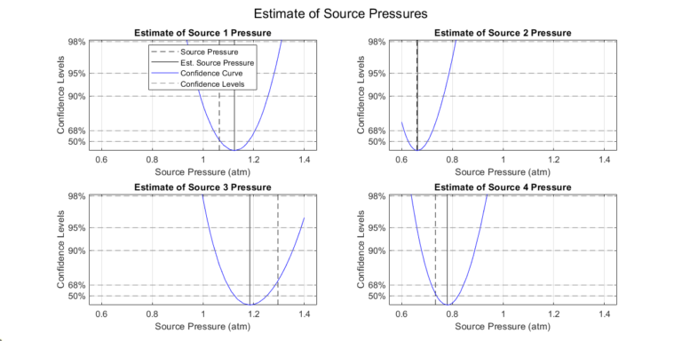
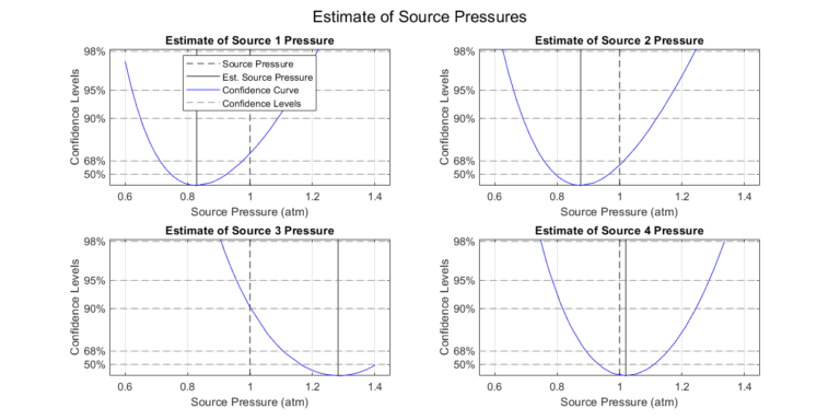
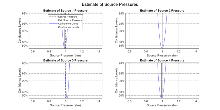
We perform the parameter estimation procedure detailed in Parameter Estimation via Profile Likelihoods. The procedure results in confidence levels for the parameter estimates. It’s important to note that the quality of the parameter estimation will directly impact the quality of the optimization. In essence, the more uncertainty present in the fixed variables, the lower the performance the optimization framework can achieve.
Step 2: Compute Source Pressure Set
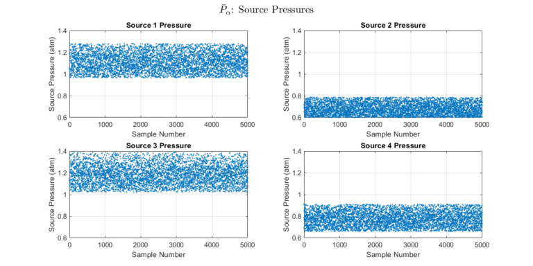
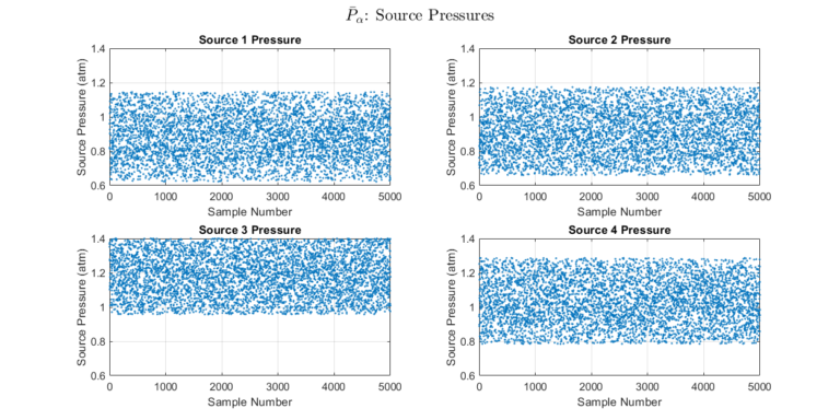
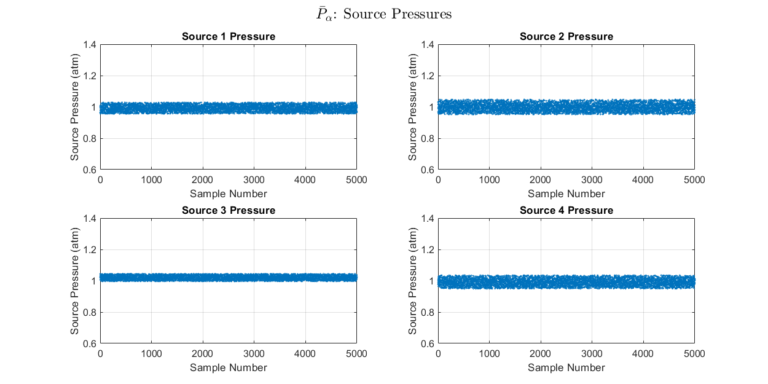
Once the confidence intervals are found, a set \( \bar{P}_\alpha \) can be constructed. A set of a specified size is computed in which members fall within the specified confidence level. We plot the gathered set for visual inspection.
Step 3: Optimize over Source Pressure Set and Validate Performance
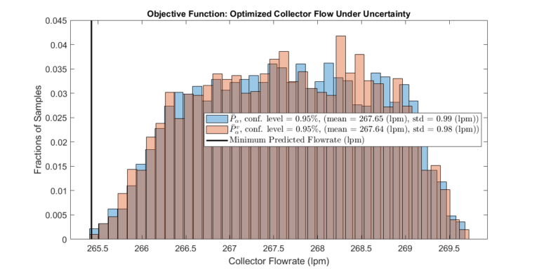
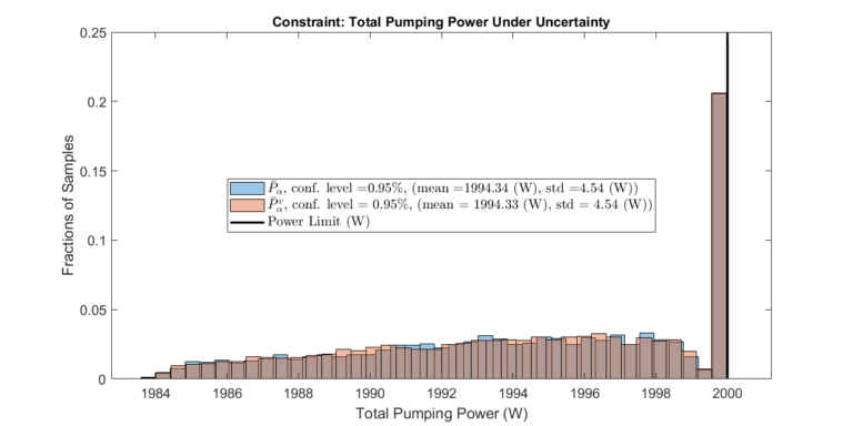
The optimization framework described above is executed. The plots below display the expected performance of the optimized system with a specific confidence level.
In addition, a validation set \( \bar{P}_\alpha^v \) is constructed to validate the optimization results. Note that \( \bar{P}_\alpha^v \) and \( \bar{P}_\alpha \) need not have the same size or confidence level. However, the validation will only make sense if the confidence level of \( \bar{P}_\alpha^v \) is equal to or less than the confidence level of \( \bar{P}_\alpha \).
Affect of Parameter Estimation Quality
As mentioned previously, parameter estimation quality directly affects the quality of the optimized solutions. We have compared two scenarios to illustrate this point. The figures below display results from two different scenarios. In the first scenario, five sensor samples are gathered, with noise models for the flow meter and pressure sensors specified as \( \mathcal{N}(0,1.5^2)\) (lpm) and \( \mathcal{N}(0,0.2^2)\) (kPa), respectively. In the second, twenty sensor samples are gathered, with noise models for the flow meter and pressure sensors specified as \( \mathcal{N}(0,0.25^2)\) (lpm) and \( \mathcal{N}(0,0.1^2)\) (kPa), respectively.
The optimization conducted on the second scenario yielded a significantly more predictable system performance. Notably, the range of possible collector flow rates is much narrower. Furthermore, the spread of possible source pressures in set \( \bar{P}_\alpha^v \) is considerably narrower in the second scenario. However, it’s crucial to note that the validation sets for both cases demonstrated the optimization framework’s ability to consistently deliver predictable results that satisfied the given constraints.
Scenario 1: Lower Accuracy Parameter Estimation
Scenario 2: Higher Accuracy Parameter Estimation
Summary
We join the parameter estimation approach introduced in Parameter Estimation via Profile Likelihoods and the surrogate model-based optimization framework discussed in Surrogate Model-Based Optimization to achieve an optimization solution under uncertain modeling parameters. Specifically, we explicitly use the parameter estimation’s confidence intervals to perform constrained optimization over a distribution of possible outcomes. As shown previously for other workflows, surrogate models and surrogate model-based optimization techniques are the critical enablers for this approach.