Model Predictive Operational Point Transition
Model Predictive Operational Point Transition
Goals
- Formulate Operational Point Transitions as Optimization Problems: We formulate an optimization problem to determine the optimal change in control settings during an operational point transition.
- Surrogate Model-Based Optimization: The surrogate optimization framework introduced here solves three operational point transition examples.
- Physics-Based Approach Comparison: We show the formulated optimization to be intractable if physics-based models are utilize
The article references a MATLAB executable notebook and code found here.
High-Level Highlights
Transitioning between operating points in a complex system can be challenging if constraints need to be adhered to. We first cast operational transitions with constraints as an optimization problem and then use the previously introduced surrogate model-based optimization framework to solve the formulated problem. The surrogate model-based optimization framework solves the problem quickly and robustly. Furthermore, we show that using a physics-based simulator for optimization will render this problem infeasible.
Operational Point Transitions
Suppose an operator would like to transition between two steady-state system operational points. If they were to change the control settings abruptly, the system may display unwanted dynamic behavior or violate safety constraints. Therefore, they may slowly and conservatively change the control settings. However, in a complex system with more than one control setting, it will be challenging to determine how multiple control settings should be changed and how they will interact.
Consider the water-pumping networks introduced in the Basics of Surrogate Model Creation to give a tangible example. The operator controls the motor speed of each pump in the system. However, they may need to ensure that the system’s flow rates or pressures do not change rapidly while transitioning between motor speeds. An operator will need deep expert knowledge for even minor adjustments to ensure system safety in a system with multiple interacting water pumps.
Formulation of the Optimization Problem
The task described above can be formulated as a series of sequential optimization problems:
\(\text{given} \ x_{\text{oper,k}} \ \text{and} \ x_{\text{oper,k}} \)
\(\min_{x_{\text{oper,k+1}}}(x_{\text{oper,k+1}}-x_{\text{oper,target}})^2\)
\(\text{subject to} \ g(\text{surrogate}(x_{\text{oper,k+1}})-\text{surrogate}(x_{\text{oper,k}}))\leq0,\)
where \(x_{\text{oper,target}}\) is the targeted (i.e., new) operational point, \(x_{\text{oper,k}}\) is the current operational point, and \(x_{\text{oper,k+1}}\) is the next intermediate operational point. The function \(g()\)describes constraints on the rate of change of system states. We solve the optimization problem sequentially to yield a chain of intermediate operational points (steps) ending with the goal operational point: \(x_{\text{oper,1}} \rightarrow x_{\text{oper,2}} \rightarrow x_{\text{oper,n}} \rightarrow x_{\text{oper,target}}\). Furthermore, it is ensured that the given constraints are not violated during each intermediate transition (e.g.\(x_{\text{oper,k}} \rightarrow x_{\text{oper,k+1}}\) ). At each step, the optimization attempts to find the largest change in the operational point that will not violate the given constraints.
Examples
Three examples of model predictive operational point transitions are described and solved. We use the surrogate model-based optimization framework to optimize quickly and robustly. Optimizations are executed with different initial seeds several times to ensure consistent and robust solutions. In practice, executions can be conducted in parallel to achieve quicker results.
The Basics of Surrogate Model Creation describes the small-scale and large-scale water pumping networks used in the following examples.
Example 1: Small-Scale with Collector Flowrate Change Limit
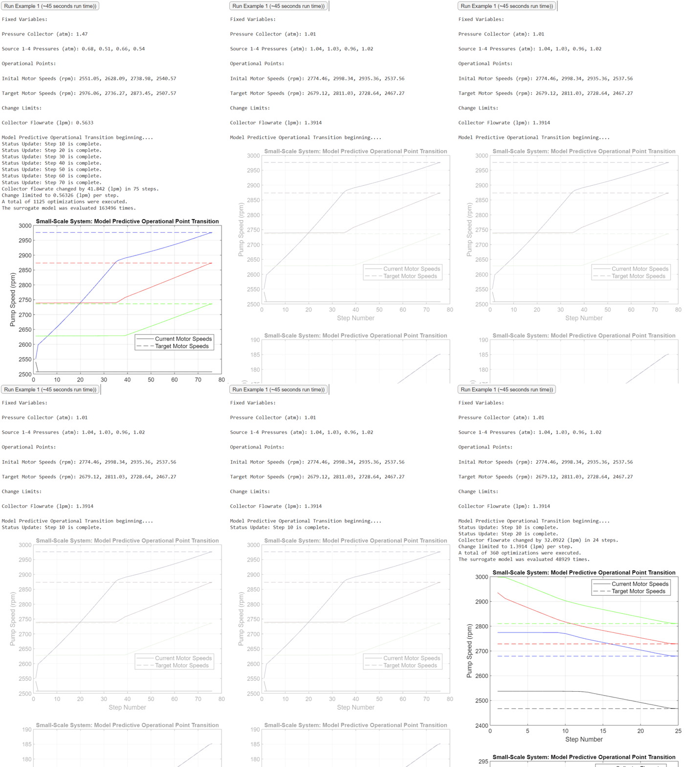
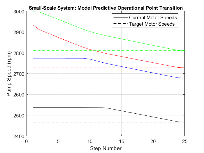
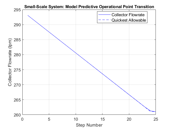
In this example, we transition the motor speeds of four pumps while ensuring the change in flow rate at the collector remains within specified limits.
In the MATLAB executable notebook, a button is used to initiate the optimization process. The initial and target points and the flow rate change limit are randomly selected. The optimization process provides a sequence of motor speeds and the expected flow rate at each intermediate transition step.
The output text also includes the number of surrogate model evaluations required. Depending on the random scenario, tens of thousands of surrogate model evaluations may be necessary. A comparison table illustrates the computational effort needed for the same number of physics-based evaluations. Notably, even for this small-scale system, performing model predictive operational point transitions using physics-based models is impractical due to the significant computational effort required. The surrogate model plays a pivotal role in enabling this workflow.
The video below displays the optimization process in action. In the example below, the optimization process executed 48,929 surrogate model evaluations to determine an optimal solution of 25 steps.

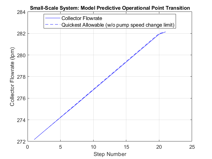
Example 2: Small-Scale with Collector Flowrate Change and Motor Speed Limits
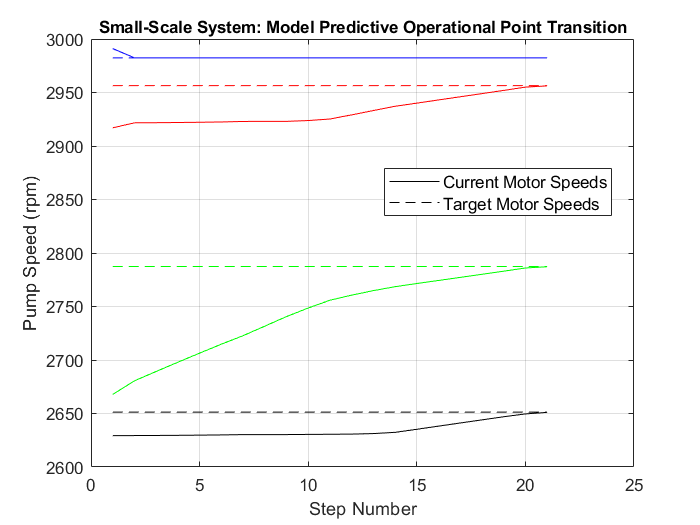
This example limits the rate of change in the motor speeds. In practice, rapidly changing a pump’s speed may not be desirable (or even possible).
In the MATLAB executable notebook, a button is used to initiate the optimization process. The initial and target operating points and the specified limits are randomly selected. The optimization process generates a sequence of motor speeds and the expected flow rate at each intermediate transition step.
Example 3: Large-Scale with Subsystem Flowrate Change Limits
The final example uses the large-scale system to demonstrate the framework’s effectiveness. We imposed limits on the flow rates of each subsystem and the collector. Recall that there are eight subsystems in the large-scale network, each consisting of multiple lines. Even for the most highly skilled operator, this high-dimensional example would be impossible to solve.
In the MATLAB executable notebook, a button is used to initiate the optimization process. The initial and target operating points and the specified limits are randomly selected.
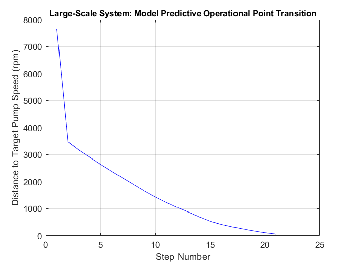
The first plot illustrates the diminishing “distance” between the current and target operational points. We define “distance” as the sum of differences between target and current speeds across all motors:
\( \sum | \omega_{\text{i,target}} – \omega_{\text{i,current}} |\)
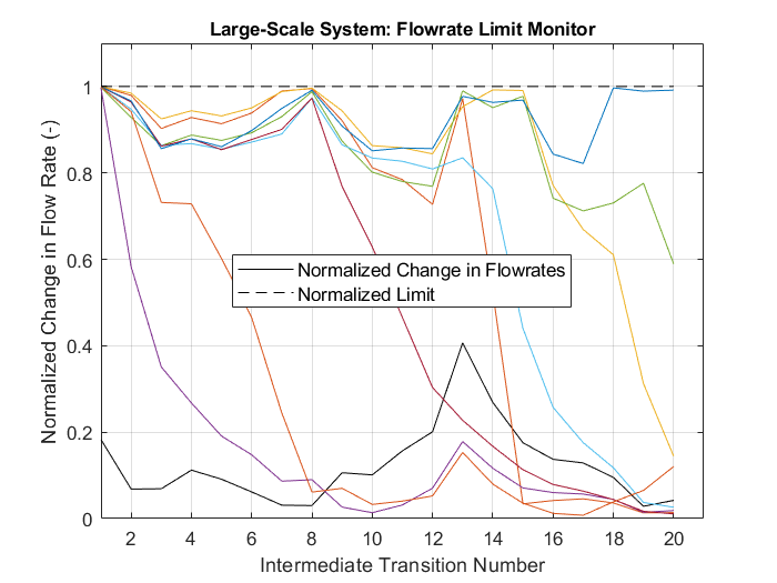
The optimization process also outputs the changes in flow rates at the collector and subsystems normalized by their respective limits. The limit was violated if a normalized flow rate change is more than 1. If the sequence of steps were perfectly efficient, then at least one normalized change in flow rate would always be equal to 1. However, due to the problem’s large dimension, the optimization process may not output a perfectly efficient answer. Nevertheless, the optimization process finds a fairly efficient sequence of steps to reach the goal operational point.
Summary
We demonstrated an exciting use case of the surrogate model-based optimization framework. As shown in example 1, using a physics-based simulator instead of a surrogate model would render this use case infeasible. This article introduces one of the many use cases that only become feasible when a quick and accurate surrogate model is available.