Basics of Surrogate Model Creation
Basics of Surrogate Model Creation
Goals
- Outline Process: Explain the fundamental steps involved in creating surrogate models of physics-based models.
- Highlight Key Benefits: Emphasize the advantages of using surrogate models, particularly their ability to predict system behavior faster than traditional physics-based models without compromising accuracy.
- Illustrate Performance Evaluation: Assess surrogate model performance, focusing on error analysis and comparisons with physics-based models.
The article references a MATLAB executable notebook found here.
High-Level Highlights
Surrogate models drastically increase the utility of physics-based models and provide a blazing-fast engine for analysis, optimization, and digital twin applications. The tables below showcase a key feature of surrogate models: they obtain answers that are nearly identical to physics-based models but in a fraction of the time.


Other articles will explore how surrogate models are leveraged to unlock novel workflows.
Physics-Based Model: Water Pumping Network Model
Model Selection
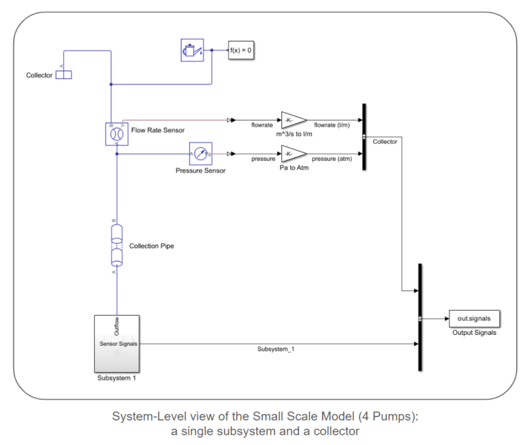
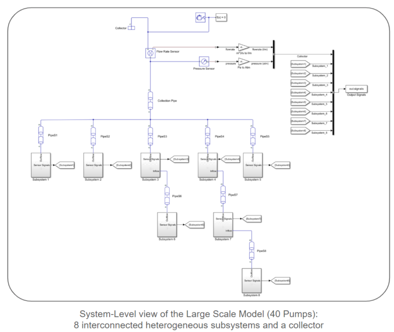
In this article, we employ two water-pumping network models to illustrate the process of surrogate model creation. We begin with a small-scale model featuring four pumps to guide readers through the essential steps. Additionally, we introduce a larger-scale model with 40 pumps to highlight the scalability of the approach. It’s important to note that our focus is solely on steady-state solutions.
Complex Dynamics of Water Pumping Networks
Water pumping networks are complex systems that exhibit coupled behavior between pumps. Simulators obtain valid solutions by resolving network pressure balance equations with iterative numerical solvers. Adjusting a single pump setting can reverberate throughout the entire network, impacting pressure and flow rate. Furthermore, the network model incorporates centrifugal pump models, capturing the intricate relationship between operating speed, flow rate, and brake power with complex pump curves.
Typically, water pumping networks are finely balanced and have additional components such as check valves to prevent backflow (water flowing back to the source). In the following, backflow is allowed since the scope of this article is to explain the basics of surrogate model creation. Therefore, some of the data collected from the physics-based model may contain undesired system behavior, but regardless, the surrogate model will accurately predict the simulated system’s behavior. A subject matter expert may carefully select the sampling bounds to prevent undesired operating conditions. Nevertheless, subsequent articles will address check valves and backflow.
Modular Structure of the Models
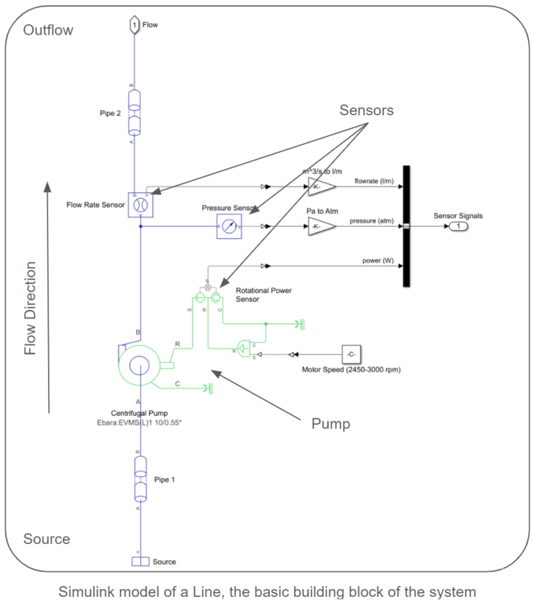
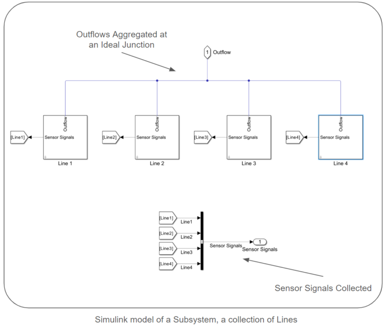
The models follow a modular structure comprised of interconnected subsystems. Each subsystem consists of a collection of lines. Each line includes a source, a pipe connecting the source to a pump, the pump itself, sensors to capture pump power, pressure, and flow rate at the pump’s outlet, and a pipe leading the flow out of the line. A collection of lines are connected via an ideal junction to create a subsystem. Pipes connect these subsystems, and a collector node is a sink for the entire network. We provide simulink models for both small and large-scale systems. The lengths and elevation gains of the pipes are considered static during surrogate model creation, as they remain constant when generating samples. However, the provided sampling scripts and models allow for easy parameter configuration. Each centrifugal pump model utilizes the pump curves of the Ebara EVMS 1 10/0.55 Vertical Multistage Pump.
Surrogate Model Scoping: Inputs and Outputs
Creating a surrogate model involves a series of steps. The first step is to identify the inputs and outputs of the model. These are usually determined based on the specific application of the surrogate model. Additionally, the inputs must be configurable in the physics-based model, and a method must be established to record the desired outputs after executing the physics-based simulation. The targetted workflow should inform the selection of input ranges. Ideally, the ranges are selected only large enough to accomplish the targeted workflow. Unnecessarily large bounds result in larger sampling and training times. We recommend automating the sampling processes to enhance efficiency (see provided code for examples).
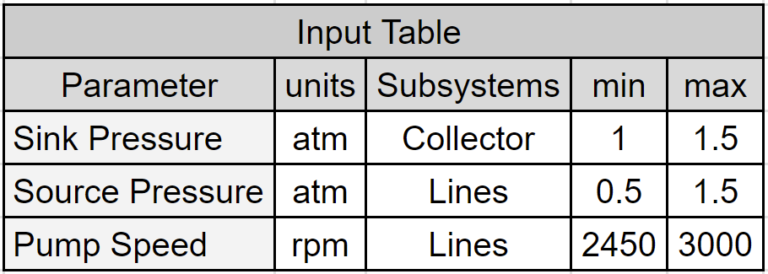
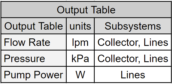
In this article, the chosen inputs for this example are source pressures, pump speeds, and the pressure at the network’s collection point (sink). Below are tables listing the inputs, their selected ranges, and the outputs collected while sampling the water-pumping network models.
Model Sampling
A total of 1000 and 8500 model samples were generated for the small-scaled and large-scale models, respectively. The sampling process involves the following steps for each sample:
- Randomizing inputs to the physics-based model
- Executing the physics-based model
- Allowing the model to reach a steady state
- Checking the model for errors
- Recording both inputs and outputs
CSV files store the recorded samples. The table below provides a snapshot of the first few parameters in the sample table. It’s important to note that inputs are randomized independently, and each subsystem has a unique source pressure and pump speed. Adopting a sampling approach with parallel model instances will reduce the time required to obtain a sample set. The “score” columns confirm that the system reached a steady state and are not training parameters.

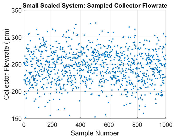
The figure below illustrates the wide range of values of the collector flow rate found in the collected samples.
Surrogate Model Generation and Deployment
We trained a surrogate model with the collected sampled set. This article uses MATLAB’s Deep Learning Toolbox [1] to train a Multilayer Perceptron (MLP) [2, 3]. The sampling set is divided into a training set (80% of samples), a validation set (10% of samples), and a testing set (10% of samples) (refer to [4] for definitions of the different sets). MAT files store the model’s parameters and structure. The provided P-code files execute inference by reconstructing surrogate models with the stored parameters and structure. The P-code functions return the MLP’s prediction of system behavior (outputs) as a function of its inputs.
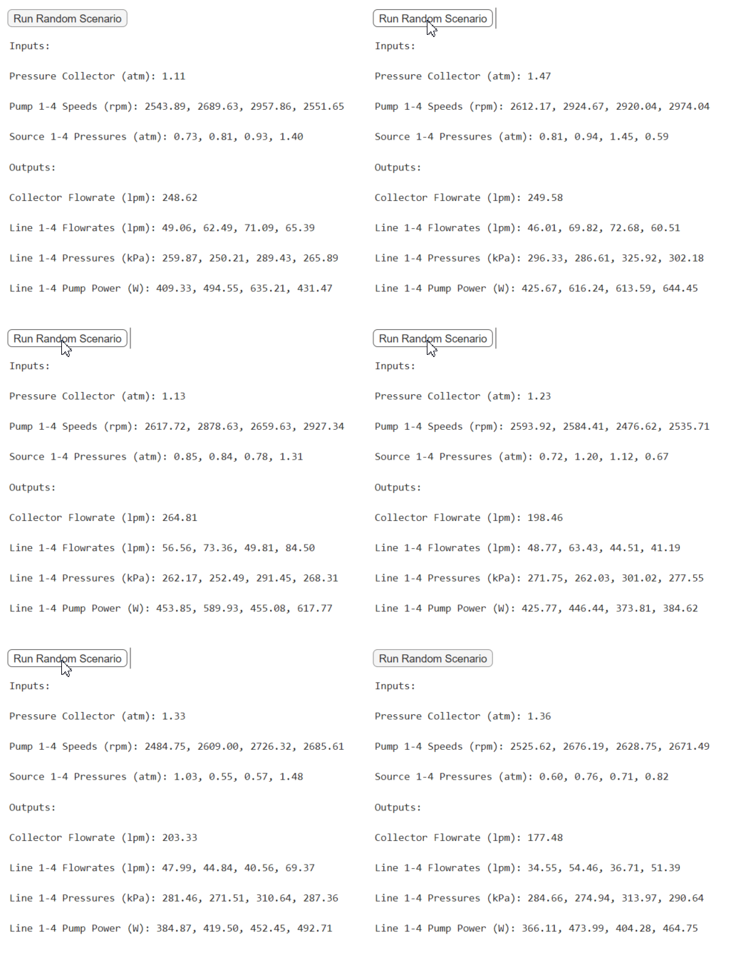
In the MATLAB executable notebook, a button is used to run a randomly selected scenario in real-time.
Surrogate Model Evaluation
Prediction Errors
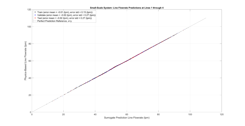
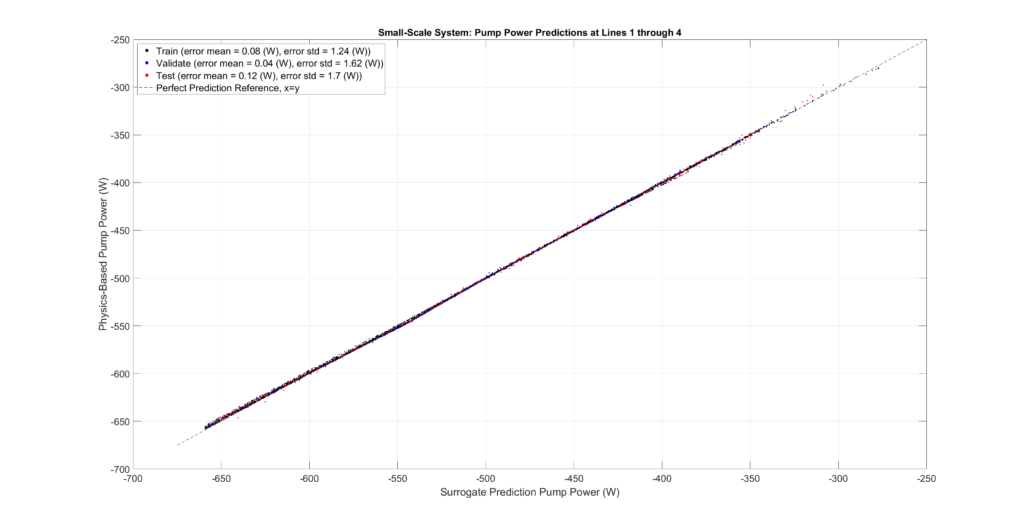
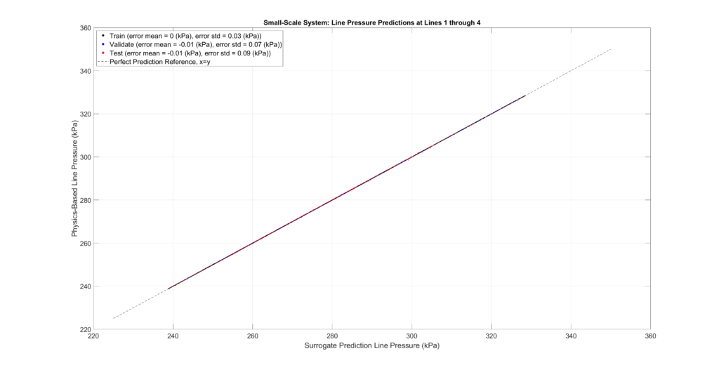
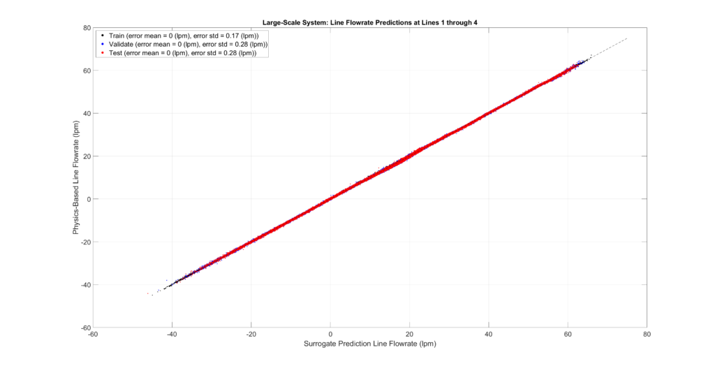
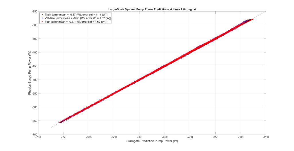
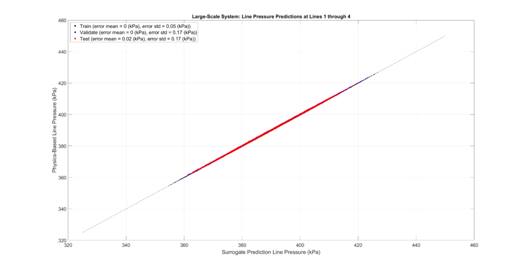
The figures below plot the surrogate predictions against the physics-based outputs for the training, validation, and testing sets. MLPs tend to be overfitted, resulting in smaller errors for the training set. Therefore, the metrics from the validation and testing sets provide a more accurate indication of errors when predicting configurations not present in the sampled set.
The tables and figures show the surrogate’s prediction error metrics (formula given below). Note that prediction errors are only a tiny fraction of the predicted values and may even be negligible in most practical applications.
\(\text{Surrogate Precent Error} = \text{Surrogate Prediction – Simulation Value}\)
Small-Scale Model Performance
Large-Scale Model Performance
Evaluation Time
Surrogate model inference occurs much quicker than executing a physics-based model. One can expect speed-ups of multiple orders of magnitude. Recall that inferencing a surrogate model is mostly a series of additions, multiplications, and simple activation functions. There are no complex physics equations to solve or keep track of. The presented surrogate will be even quicker with more efficient deployments.
In the MATLAB executable notebook, slide bars are used to select the number of samples to test for a speed time evaluation. We conducted two assessments. The first evaluates the speed of the surrogate to perform inference in series for single system configurations. The second considers the surrogate inference to perform a batch inference.

Summary
The tables below (the same ones shown in High-Level Highlights) offer a performance comparison between the surrogate model and the physics-based models. Surrogate models significantly reduce execution time by orders of magnitude while introducing only minor errors into the system’s predictions. Further reduction in surrogate model execution time is achievable with more time-efficient deployments. Notably, the reduction in execution time is more pronounced in the large-scale model.

